完整课程

简介

什么是 sklearn？

Scikit-learn（通常简称为 sklearn）是一个用于 Python 的机器学习库。它基于 NumPy、SciPy 和 matplotlib 构建，提供了丰富的工具集，用于数据挖掘和数据分析，特别适合进行小规模和中等规模的机器学习项目。

官方将 sklearn 描述为：

简单高效的数据挖掘和数据分析工具
可供大家在各种环境中重复使用
建立在 NumPy ，SciPy 和 matplotlib 上
开源，可商业使用 - BSD 许可证

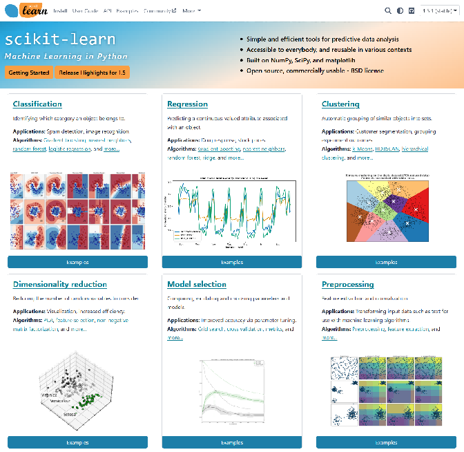
sklearn 的主要功能

分类: 识别数据类别并预测新的数据点属于哪个类别，例如垃圾邮件检测。
回归: 预测目标变量的值，例如预测房价。
聚类: 自动将相似数据分组，例如客户群体划分。
降维: 降低数据维度以便于可视化或减少计算量，例如 PCA（主成分分析）。
模型选择: 用于选择模型参数、交叉验证等，例如网格搜索。
预处理: 数据标准化、归一化等，准备数据用于机器学习。

为什么选择 sklearn？

易于使用: API 设计直观，易于上手。
丰富的文档和社区支持: 官方文档详细，社区活跃，提供了大量的学习资源。
与 Python 生态系统兼容: 可以与其他 Python 库（如 Pandas、NumPy、matplotlib）无缝集成。

环境搭建

TIP

详细教程：Anaconda 环境搭建

安装 Anaconda

在 Anaconda 安装的过程中，比较容易出错的环节是环境变量的配置，所以大家在配置环境变量的时候，要细心一些。

双击下载好的安装包，点击 Next，点击 I Agree，选择 Just Me，选择安装路经（安装在 C 盘也有好处，不过与 C 盘爆炸来说不值一提，建议按在其他盘）然后 Next，来到如下界面：

请选择 Register Anaconda as my default Python 3.x，不要选 Add Anaconda to my PATH environment variable，我们需要后期手动添加环境变量。

点击 Install，安装需要等待一会儿。

最后一直 Next，直到安装完成。

对于两个“learn”，都取消打勾，不用打开去看了，耽误时间。

安装好后我们需要手动配置环境变量。

配置环境变量

计算机（右键）→ 属性 → 高级系统设置 →（点击）环境变量

在下面系统变量里，找到并点击 Path

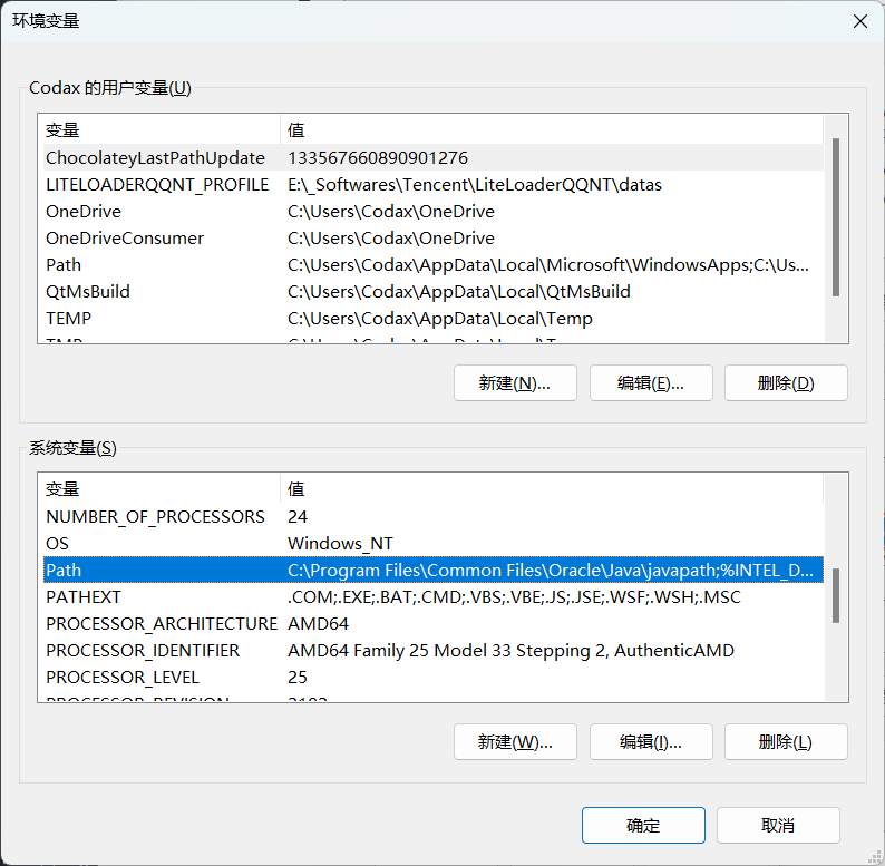
在编辑环境变量里，点击新建

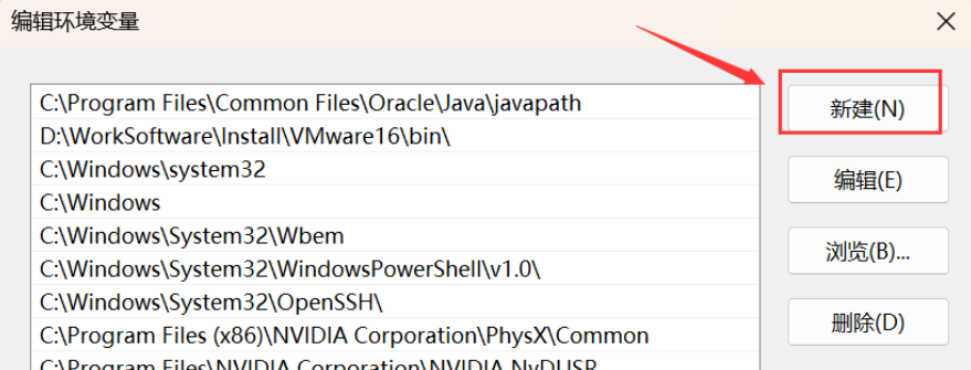
输入下面的五个环境变量。（这里不是完全一样的！你需要将以下五条环境变量中涉及的到的"D:\_Producers\Anaconda3"都修改为你的 Anaconda 的安装路径！）

D:\_Producers\Anaconda3
D:\_Producers\Anaconda3\Scripts
D:\_Producers\Anaconda3\Library\bin
D:\_Producers\Anaconda3\Library\mingw-w64\bin
D:\_Producers\Anaconda3\Library\usr\bin

简要说明五条路径的用途：这五个环境变量中，1 是 Python 需要，2 是 conda 自带脚本，3 是 jupyter notebook 动态库, 4 是使用 C with python 的时候

新建完成后点击确定。

验证

打开 cmd，在弹出的命令行查看 anaconda 版本，依次输入：

shell

conda --version
python --version

若各自出现版本号，即代表配置成功。

在开始菜单或桌面找到 Anaconda Navifator 将其打开（若桌面没有可以发一份到桌面，方便后续使用），出现 GUI 界面即为安装成功。

更改 conda 源

如果你没有魔法上网工具，建议更改 conda 源，这样可以加快下载包的速度。清华大学提供了 Anaconda 的镜像仓库，我们把源改为清华大学镜像源。

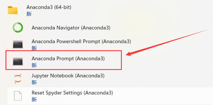
找到 Anaconda prompt，打开 shell 面板。

在命令行输入以下命令：

shell

conda config --add channels https://mirrors.tuna.tsinghua.edu.cn/anaconda/pkgs/free/
conda config --add channels https://mirrors.tuna.tsinghua.edu.cn/anaconda/cloud/conda-forge
conda config --add channels https://mirrors.tuna.tsinghua.edu.cn/anaconda/cloud/msys2/
conda config --set show_channel_urls yes

查看是否修改好通道：

shell

conda config --show channels

安装相关 Python 库

Anaconda 自带了一些常用的机器学习库，如 numpy、pandas、matplotlib、seaborn、scikit-learn 等。

如果需要安装其他库，可以直接在 Anaconda Navigator 里搜索安装。

Hello, Sklearn!

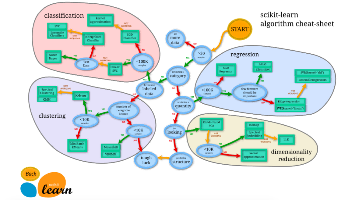
机器学习方法

对于任何一个问题，如果我们希望通过机器学习的方式解决，我们一般遵循以下步骤：

问题分析：我们需要清楚问题的类型、输入、输出、数据集、目标、评估指标等。
数据预处理：我们需要对数据进行清洗、转换、归一化等操作，确保数据质量。
训练模型：我们需要选择合适的机器学习算法，并训练模型。
预测与评估：我们需要使用测试集对模型进行测试，并评估模型的性能。

如果我们决定好了用哪些方法进行机器学习，我们可以在官方文档中找到相应的 API，按照接口一步步实现。

接下来，我们从一个简单的 KNN 模型入手，配合经典的 Iris 数据集，来熟悉 sklearn 的使用。

KNN 算法简介

K-近邻算法是一种有监督学习、分类（也可用于回归）算法。

TIP

可以在这里查看完整的 KNN 算法教程：K-近邻算法(KNN)

K Nearest Neighbor 算法又叫 KNN 算法，它假设如果一个样本在特征空间中的 k 个最相似(即特征空间中最邻近)的样本中的大多数属于某一个类别，则该样本也属于这个类别。

KNN 算法的流程如下：

计算已知类别数据集中的点与当前点之间的欧式距离
按距离递增次序排序
选取与当前点距离最小的 k 个点
统计前 k 个点所在的类别出现的频率
返回前 k 个点出现频率最高的类别作为当前点的预测分类

sklearn 中 KNN 算法的 API 如下：

python

sklearn.neighbors.KNeighborsClassifier(n_neighbors=3, weights='uniform', algorithm='auto', leaf_size=30, p=2, metric='minkowski', metric_params=None, n_jobs=None)

其中：

n_neighbors：选择最近邻的数目，默认为 3。
weights：选择样本权重的方法，默认为 uniform，即所有样本权重相同。
algorithm：选择计算最近邻的方法，默认为 auto，即自动选择。
leaf_size：设置叶子节点的大小，默认为 30。
p：选择距离度量的指数，默认为 2。
metric：选择距离度量的方法，默认为 minkowski，即闵可夫斯基距离。
metric_params：设置距离度量的参数，默认为 None。
n_jobs：设置并行计算的线程数，默认为 None，即自动选择。

问题分析

假设我们有一组关于鸢尾花的特征数据，包括花萼长度、花萼宽度、花瓣长度、花瓣宽度、类别（山鸢尾、变色鸢尾、维吉尼亚鸢尾）等特征。当有一组新的数据时，我们希望通过这一组的数据预测鸢尾花的类别。

具体的数据及其引入方法如下：

python

from sklearn.datasets import load_iris
import pandas as pd

# 导入数据集
iris = load_iris()
# print(iris)
iris_df = pd.DataFrame(iris.data, columns=iris.feature_names)
iris_df['species'] = iris.target
print(iris_df.head())

输出结果：

shell

   sepal length (cm)  sepal width (cm)  petal length (cm)  petal width (cm)  species
0                5.1               3.5                1.4               0.2        0
1                4.9               3.0                1.4               0.2        0
2                4.7               3.2                1.3               0.2        0
3                4.6               3.1                1.5               0.2        0
4                5.0               3.6                1.4               0.2        0

分析：

输入：鸢尾花的特征数据，包括花萼长度、花萼宽度、花瓣长度、花瓣宽度。
输出：鸢尾花的类别，包括山鸢尾、变色鸢尾、维吉尼亚鸢尾。
目标：预测新数据属于哪个类别。
评估指标：准确率。

我们可以绘制一个图形来进一步观察数据的特征：

python

import matplotlib.pyplot as plt

# 可视化数据集
plt.figure(figsize=(10, 6))
plt.xlabel('sepal length (cm)')
plt.ylabel('sepal width (cm)')
plt.scatter(iris_df[iris_df['species'] == 0]['sepal length (cm)'], iris_df[iris_df['species'] == 0]['sepal width (cm)'], color='red', label='Setosa')
plt.scatter(iris_df[iris_df['species'] == 1]['sepal length (cm)'], iris_df[iris_df['species'] == 1]['sepal width (cm)'], color='green', label='Versicolor')
plt.scatter(iris_df[iris_df['species'] == 2]['sepal length (cm)'], iris_df[iris_df['species'] == 2]['sepal width (cm)'], color='blue', label='Virginica')
plt.legend()
plt.title('Iris Dataset - Sepal Length vs Width')
plt.show()

输出结果：

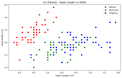
从图中我们可以看出，相同种类的鸢尾花其特征数据之间的距离较近，而不同种类的鸢尾花，其特征数据之间的距离较远。因此，KNN 算法是一种可能解决此问题的有效方案。

数据预处理

通常我们获得的数据都是不完美的，需要进行数据预处理，一般使用以下方法：

特征工程（Feature Engineering）：特征工程是指从原始数据中提取有用的特征，并将其转换为适合机器学习算法的形式。
数据清洗（Data Cleaning）：数据清洗是指对数据进行检查、修复、过滤、转换等操作，以确保数据质量。
数据转换（Data Transformation）：数据转换是指对数据进行变换，以便更好地适应机器学习算法。
数据集成（Data Integration）：数据集成是指将不同来源的数据进行整合，以便更好地训练模型。

在这里，我们先仅作最简单的标准化处理。

TIP

如果想了解更多关于数据预处理的方法，可以查看特征工程-特征预处理

具体的标准化方法如下：

sklearnpython

python

from sklearn.preprocessing import StandardScaler

# 数据预处理
scaler = StandardScaler()
x = scaler.fit_transform(iris.data)

python

# 手动实现标准化
class MyStandardScaler:
    def __init__(self):
        self.mean_ = None
        self.scale_ = None

    def fit(self, X):
        """
        计算并存储数据的均值和标准差

        参数:
        X: 输入数据，形状为 (n_samples, n_features)

        返回:
        self: 返回自身的引用
        """
        self.mean_ = np.mean(X, axis=0)
        self.scale_ = np.std(X, axis=0)
        return self

    def transform(self, X):
        """
        根据存储的均值和标准差对数据进行标准化

        参数:
        X: 输入数据，形状为 (n_samples, n_features)

        返回:
        X_scaled: 标准化后的数据，形状为 (n_samples, n_features)
        """
        if self.mean_ is None or self.scale_ is None:
            raise ValueError("Scaler has not been fitted yet.")
        X_scaled = (X - self.mean_) / self.scale_
        return X_scaled

    def fit_transform(self, X):
        """
        计算均值和标准差，并对数据进行标准化

        参数:
        X: 输入数据，形状为 (n_samples, n_features)

        返回:
        X_scaled: 标准化后的数据，形状为 (n_samples, n_features)
        """
        return self.fit(X).transform(X)


# 数据预处理
scaler = StandardScaler()
x = scaler.fit_transform(iris.data)

python

# 对比预处理效果（可选）
plt.figure(figsize=(12, 5))
plt.subplot(1, 2, 1)
plt.hist(iris.data[:, 0], bins=20, color='blue', alpha=0.7)
plt.title('Before Scaling')
plt.subplot(1, 2, 2)
plt.hist(x[:, 0], bins=20, color='green', alpha=0.7)
plt.title('After Scaling')
plt.show()

输出结果：

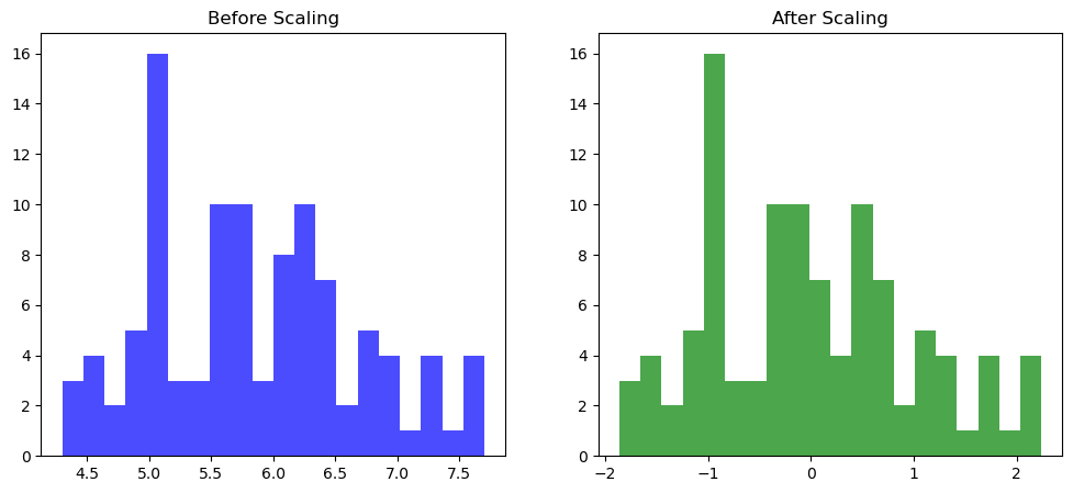
从图中我们可以看出，数据标准化 使得数据分布变得更加均匀，更容易被模型识别。（虽然本案例中的原始数据集已经够匀称了）

划分数据集

机器学习是从数据的属性中学习，并将它们应用到新数据的过程。这就是为什么机器学习中评估算法的普遍实践是把数据分割成 训练集 （我们从中学习数据的属性）和 测试集 （我们测试这些性质）。在这里，我们简单把数据集按 7:3 切分为训练集和测试集。

TIP

如果你想了解更多关于数据集、拟合、误差等知识，可以查看拆分原始训练集

具体的切分方法如下：

sklearnpython

python

from sklearn.model_selection import train_test_split

# 切分数据集
x_train, x_test, y_train, y_test = train_test_split(x, iris.target, test_size=0.3, random_state=42)
print(f"Training set size: {x_train.shape}, {y_train.shape}")
print(f"Testing set size: {x_test.shape}, {y_test.shape}")

python

import numpy as np

# 手动实现数据集划分
def train_test_split(X, y, test_size=0.3, random_state=None):
    """
    将数据集划分为训练集和测试集

    参数:
    X: 样本特征，形状为 (n_samples, n_features)
    y: 样本标签，形状为 (n_samples,)
    test_size: 测试集所占比例，范围为 (0, 1) 之间
    random_state: 随机种子，确保结果可复现

    返回:
    X_train, X_test, y_train, y_test: 分别为训练集和测试集的特征和标签
    """

    # 设置随机种子以确保可复现性
    if random_state is not None:
        np.random.seed(random_state)

    # 获取样本数量
    n_samples = X.shape[0]

    # 计算测试集样本数量
    n_test_samples = int(n_samples * test_size)

    # 随机打乱索引
    shuffled_indices = np.random.permutation(n_samples)

    # 划分训练集和测试集的索引
    test_indices = shuffled_indices[:n_test_samples]
    train_indices = shuffled_indices[n_test_samples:]

    # 划分训练集和测试集
    X_train = X[train_indices]
    X_test = X[test_indices]
    y_train = y[train_indices]
    y_test = y[test_indices]

    return X_train, X_test, y_train, y_test


# 划分数据集
x_train, x_test, y_train, y_test = train_test_split(x, iris.target, test_size=0.3, random_state=42)
print(f"Training set size: {x_train.shape}, {y_train.shape}")
print(f"Testing set size: {x_test.shape}, {y_test.shape}")

输出结果：

shell

Training set size: (105, 4), (105,)
Test set size: (45, 4), (45,)

训练与预测

根据我们之前的分析，我们可以选择 KNN 算法作为模型。在实际使用 KNN 模型时，我们一般通过遍历的方法来确定最优的 K 值。

sklearnpython

python

from sklearn.neighbors import KNeighborsClassifier
from sklearn.metrics import accuracy_score

# 训练模型，循环遍历不同k值，训练模型并预测测试集
accuracies = []
k_values = range(1, 11)
for k in k_values:
    knn = KNeighborsClassifier(n_neighbors=k)
    knn.fit(x_train, y_train)
    y_pred = knn.predict(x_test)
    accuracies.append(accuracy_score(y_test, y_pred))  # 模型的准确率
print(accuracies)

python

# 手动实现 KNN 算法
class MyKNN:
    def __init__(self, n_neighbors=3):
        self.n_neighbors = n_neighbors

    def fit(self, X, y):
        """
        训练KNN模型，存储训练数据

        参数:
        X: 训练样本特征，形状为 (n_samples, n_features)
        y: 训练样本标签，形状为 (n_samples,)

        返回:
        self: 返回自身的引用
        """
        self.X_train = np.array(X)
        self.y_train = np.array(y)
        return self

    def predict(self, X):
        """
        使用KNN模型进行预测

        参数:
        X: 测试样本特征，形状为 (n_samples, n_features)

        返回:
        y_pred: 预测标签，形状为 (n_samples,)
        """
        X = np.array(X)
        y_pred = np.zeros(X.shape[0])

        for i in range(X.shape[0]):
            # 计算欧氏距离
            distances = np.sqrt(np.sum((self.X_train - X[i, :])**2, axis=1))
            # 找到最近的k个点的索引
            nearest_neighbors = np.argsort(distances)[:self.n_neighbors]
            # 找到最近邻的标签
            nearest_labels = self.y_train[nearest_neighbors]
            # 投票决定预测标签
            y_pred[i] = np.argmax(np.bincount(nearest_labels))

        return y_pred

    def score(self, X, y):
        """
        计算模型在测试集上的准确率

        参数:
        X: 测试样本特征，形状为 (n_samples, n_features)
        y: 测试样本标签，形状为 (n_samples,)

        返回:
        accuracy: 测试集上的准确率
        """
        y_pred = self.predict(X)
        accuracy = np.mean(y_pred == y)
        return accuracy

# 训练模型
accuracies = []
k_values = range(1, 11)
for k in k_values:
    knn = MyKNN(n_neighbors=k)
    knn.fit(x_train, y_train)
    accuracies.append(knn.score(x_test, y_test))  # 模型的准确率
print(accuracies)

输出结果：

shell

[0.9777777777777777, 0.9777777777777777, 1.0, 0.9777777777777777, 1.0, 1.0, 1.0, 1.0, 1.0, 1.0]

我们可以画一个折线图来展示 K 值与准确率之间的关系：

python

# 绘制准确率与k值的关系图（可选）
plt.figure(figsize=(10, 6))
plt.plot(k_values, accuracies, marker='o')
plt.xlabel('K Value')
plt.ylabel('Accuracy')
plt.title('K Value vs. Accuracy')
plt.grid()
plt.show()

输出结果：

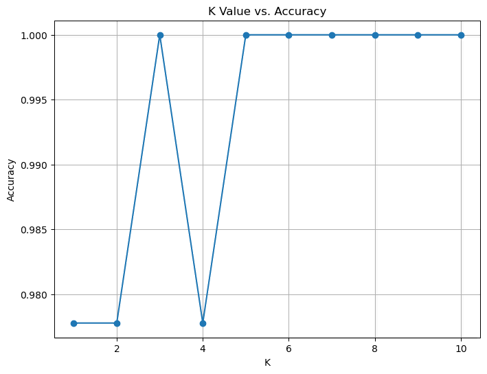
由于数据集质量较好，可以看到 KNN 的取值在各个值下都有较好的准确率。不过在 K≥5 时，准确率一直维持在较高水平，因此我们可以选择 K=6 作为最终的模型：

sklearnpython

python

# 确定模型
knn = KNeighborsClassifier(n_neighbors=5)
knn.fit(x_train, y_train)

# 预测测试集
y_pred = knn.predict(x_test)
for i in range(5):
    print(f"True label: {y_test[i]}, Predicted label: {y_pred[i]}")

python

# 确定模型
knn = MyKNN(n_neighbors=5)
knn.fit(x_train, y_train)

# 预测测试集
y_pred = knn.predict(x_test)
for i in range(5):
    print(f"True label: {y_test[i]}, Predicted label: {y_pred[i]}")

输出结果：

shell

True label: 1, Predicted label: 1
True label: 0, Predicted label: 0
True label: 2, Predicted label: 2
True label: 1, Predicted label: 1
True label: 1, Predicted label: 1

模型评估

我们可以通过一些指标来评估模型的性能，常用的指标有：

准确率（Accuracy）：正确分类的样本数与总样本数的比值。
精确率（Precision）：正确分类为正的样本数与所有正样本数的比值。
召回率（Recall）：正确分类为正的样本数与所有样本中正样本的比值。
F1 值（F1 Score）：精确率和召回率的调和平均值。
混淆矩阵（Confusion Matrix）：用于描述分类结果的矩阵。

TIP

如果想了解更多关于模型评估的方法，可以查看分类评估

这里我们使用准确率、评估报告（包含精确率、召回率、F1 值、支持）与混淆矩阵来进行简单评估：

sklearnpython

python

from sklearn.metrics import accuracy_score, classification_report, confusion_matrix

# 计算准确率
accurancy = accuracy_score(y_test, y_pred)
print(f"Accuracy: {accurancy:.2f}")

# 计算分类报告
report = classification_report(y_test, y_pred)
print(report)

# 计算混淆矩阵
cm = confusion_matrix(y_test, y_pred)
print(cm)

python

# 手动实现精准率
def accuracy_score(y_true, y_pred):
    """
    计算准确率

    参数:
    y_true: 真实标签，形状为 (n_samples,)
    y_pred: 预测标签，形状为 (n_samples,)

    返回:
    accuracy: 准确率（浮点数）
    """
    correct_predictions = np.sum(y_true == y_pred)
    accuracy = correct_predictions / len(y_true)
    return accuracy


# 手动实现分类报告
def classification_report(y_true, y_pred, target_names=None):
    """
    计算分类报告，包括精确率、召回率和 F1 分数

    参数:
    y_true: 真实标签，形状为 (n_samples,)
    y_pred: 预测标签，形状为 (n_samples,)
    target_names: 类别名称列表（可选）

    返回:
    report: 分类报告字符串
    """
    labels = np.unique(y_true)
    if target_names is None:
        target_names = [str(label) for label in labels]

    report = "               precision    recall  f1-score   support\n"
    report += "\n"

    for i, label in enumerate(labels):
        tp = np.sum((y_true == label) & (y_pred == label))
        fp = np.sum((y_true != label) & (y_pred == label))
        fn = np.sum((y_true == label) & (y_pred != label))

        precision = tp / (tp + fp) if (tp + fp) > 0 else 0.0
        recall = tp / (tp + fn) if (tp + fn) > 0 else 0.0
        f1 = 2 * precision * recall / (precision + recall) if (precision + recall) > 0 else 0.0
        support = np.sum(y_true == label)

        report += f"{target_names[i]:>15}   {precision:>9.2f}   {recall:>6.2f}   {f1:>8.2f}   {support:>7}\n"

    return report


# 手动实现混淆矩阵
def confusion_matrix(y_true, y_pred):
    """
    计算混淆矩阵

    参数:
    y_true: 真实标签，形状为 (n_samples,)
    y_pred: 预测标签，形状为 (n_samples,)

    返回:
    cm: 混淆矩阵，形状为 (n_classes, n_classes)
    """
    labels = np.unique(y_true)
    cm = np.zeros((len(labels), len(labels)), dtype=int)

    for i, label_true in enumerate(labels):
        for j, label_pred in enumerate(labels):
            cm[i, j] = np.sum((y_true == label_true) & (y_pred == label_pred))

    return cm


# 计算准确率
accurancy = accuracy_score(y_test, y_pred)
print(f"Accuracy: {accurancy:.2f}")

# 计算分类报告
report = classification_report(y_test, y_pred)
print(report)

# 计算混淆矩阵
cm = confusion_matrix(y_test, y_pred)
print(cm)

输出结果：

shell

Accuracy: 1.00
              precision    recall  f1-score   support

           0       1.00      1.00      1.00        19
           1       1.00      1.00      1.00        13
           2       1.00      1.00      1.00        13

    accuracy                           1.00        45
   macro avg       1.00      1.00      1.00        45
weighted avg       1.00      1.00      1.00        45

[[19  0  0]
 [ 0 13  0]
 [ 0  0 13]]

可以看到预测结果的准确率、精确率、召回率、F1 值都达到了 1.0，说明模型完全拟合测试集。

我们可以绘制一个混淆矩阵图来更直观地展示分类结果：

sklearnpython

python

from sklearn.metrics import ConfusionMatrixDisplay

# 绘制混淆矩阵热力图（可选）
cm_display = ConfusionMatrixDisplay(cm, display_labels=iris.target_names)
cm_display.plot(cmap=plt.cm.Blues)
plt.title('Confusion Matrix')
plt.show()

python

# 手动实现绘制混淆矩阵热力图
def plot_confusion_matrix(cm, target_names):
    """
    绘制混淆矩阵热力图

    参数:
    cm: 混淆矩阵，形状为 (n_classes, n_classes)
    target_names: 类别名称列表
    """
    fig, ax = plt.subplots(figsize=(8, 8))
    cax = ax.matshow(cm, cmap=plt.cm.Blues)
    plt.title('Confusion Matrix')
    fig.colorbar(cax)

    # 添加标签
    ax.set_xticks(np.arange(len(target_names)))
    ax.set_yticks(np.arange(len(target_names)))
    ax.set_xticklabels(target_names)
    ax.set_yticklabels(target_names)

    # 旋转 x 轴标签
    plt.xticks(rotation=45)

    # 添加文本标签
    for i in range(len(target_names)):
        for j in range(len(target_names)):
            ax.text(j, i, cm[i, j], ha='center', va='center', color='black')

    plt.xlabel('Predicted label')
    plt.ylabel('True label')
    plt.show()


# 绘制混淆矩阵热力图
plot_confusion_matrix(cm, iris.target_names)

输出结果：

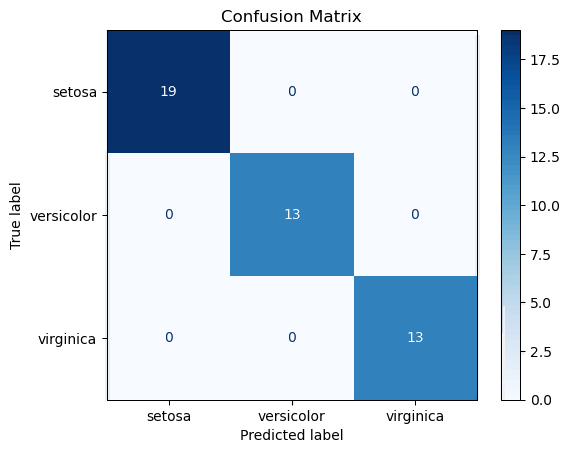
可以看到预测值与真实值完全吻合。

至此，我们完成了一个简单的 KNN 模型的训练与预测。

完整代码

sklearnpython

python

from sklearn.datasets import load_iris
from sklearn.model_selection import train_test_split
from sklearn.preprocessing import StandardScaler
from sklearn.neighbors import KNeighborsClassifier
from sklearn.metrics import accuracy_score, classification_report, confusion_matrix, ConfusionMatrixDisplay
import pandas as pd
import matplotlib.pyplot as plt

# 导入数据集
iris = load_iris()
# print(iris)
iris_df = pd.DataFrame(iris.data, columns=iris.feature_names)
iris_df['species'] = iris.target
print(iris_df.head())

# 可视化数据集
plt.figure(figsize=(10, 6))
plt.xlabel('sepal length (cm)')
plt.ylabel('sepal width (cm)')
plt.scatter(iris_df[iris_df['species'] == 0]['sepal length (cm)'], iris_df[iris_df['species'] == 0]['sepal width (cm)'], color='red', label='Setosa')
plt.scatter(iris_df[iris_df['species'] == 1]['sepal length (cm)'], iris_df[iris_df['species'] == 1]['sepal width (cm)'], color='green', label='Versicolor')
plt.scatter(iris_df[iris_df['species'] == 2]['sepal length (cm)'], iris_df[iris_df['species'] == 2]['sepal width (cm)'], color='blue', label='Virginica')
plt.legend()
plt.title('Iris Dataset - Sepal Length vs Width')
plt.show()

# 数据预处理
scaler = StandardScaler()
x = scaler.fit_transform(iris.data)

# 对比预处理效果
plt.figure(figsize=(12, 5))
plt.subplot(1, 2, 1)
plt.hist(iris.data[:, 0], bins=20, color='blue', alpha=0.7)
plt.title('Before Scaling')
plt.subplot(1, 2, 2)
plt.hist(x[:, 0], bins=20, color='green', alpha=0.7)
plt.title('After Scaling')
plt.show()

# 切分数据集
x_train, x_test, y_train, y_test = train_test_split(x, iris.target, test_size=0.3, random_state=42)
print(f"Training set size: {x_train.shape}, {y_train.shape}")
print(f"Testing set size: {x_test.shape}, {y_test.shape}")

# 训练模型
accuracies = []
k_values = range(1, 11)
for k in k_values:
    knn = KNeighborsClassifier(n_neighbors=k)
    knn.fit(x_train, y_train)
    y_pred = knn.predict(x_test)
    accuracies.append(accuracy_score(y_test, y_pred))  # 模型的准确率
print(accuracies)

# 绘制准确率与k值的关系图
plt.figure(figsize=(10, 6))
plt.plot(k_values, accuracies, marker='o')
plt.xlabel('K Value')
plt.ylabel('Accuracy')
plt.title('K Value vs. Accuracy')
plt.grid()
plt.show()

# 确定模型
knn = KNeighborsClassifier(n_neighbors=5)
knn.fit(x_train, y_train)

# 预测测试集
y_pred = knn.predict(x_test)
for i in range(5):
    print(f"True label: {y_test[i]}, Predicted label: {y_pred[i]}")

# 计算准确率
accurancy = accuracy_score(y_test, y_pred)
print(f"Accuracy: {accurancy:.2f}")

# 计算分类报告
report = classification_report(y_test, y_pred)
print(report)

# 计算混淆矩阵
cm = confusion_matrix(y_test, y_pred)
print(cm)

# 绘制混淆矩阵热力图
cm_display = ConfusionMatrixDisplay(cm, display_labels=iris.target_names)
cm_display.plot(cmap=plt.cm.Blues)
plt.title('Confusion Matrix')
plt.show()

python

# 为方便展示逻辑连贯性，函数和类的实现按顺序放在了代码中间。按照 Python 代码的习惯，在实际代码中，函数和类的实现应该放在文件开头或单独封装成模块。
from sklearn.datasets import load_iris
import pandas as pd
import matplotlib.pyplot as plt
import numpy as np

# 导入数据集
iris = load_iris()
# print(iris)
iris_df = pd.DataFrame(iris.data, columns=iris.feature_names)
iris_df['species'] = iris.target
print(iris_df.head())


# 可视化数据集
plt.figure(figsize=(10, 6))
plt.xlabel('sepal length (cm)')
plt.ylabel('sepal width (cm)')
plt.scatter(iris_df[iris_df['species'] == 0]['sepal length (cm)'], iris_df[iris_df['species'] == 0]['sepal width (cm)'], color='red', label='Setosa')
plt.scatter(iris_df[iris_df['species'] == 1]['sepal length (cm)'], iris_df[iris_df['species'] == 1]['sepal width (cm)'], color='green', label='Versicolor')
plt.scatter(iris_df[iris_df['species'] == 2]['sepal length (cm)'], iris_df[iris_df['species'] == 2]['sepal width (cm)'], color='blue', label='Virginica')
plt.legend()
plt.title('Iris Dataset - Sepal Length vs Width')
plt.show()


# 手动实现数据集划分
def train_test_split(X, y, test_size=0.3, random_state=None):
    """
    将数据集划分为训练集和测试集

    参数:
    X: 样本特征，形状为 (n_samples, n_features)
    y: 样本标签，形状为 (n_samples,)
    test_size: 测试集所占比例，范围为 (0, 1) 之间
    random_state: 随机种子，确保结果可复现

    返回:
    X_train, X_test, y_train, y_test: 分别为训练集和测试集的特征和标签
    """

    # 设置随机种子以确保可复现性
    if random_state is not None:
        np.random.seed(random_state)

    # 获取样本数量
    n_samples = X.shape[0]

    # 计算测试集样本数量
    n_test_samples = int(n_samples * test_size)

    # 随机打乱索引
    shuffled_indices = np.random.permutation(n_samples)

    # 划分训练集和测试集的索引
    test_indices = shuffled_indices[:n_test_samples]
    train_indices = shuffled_indices[n_test_samples:]

    # 划分训练集和测试集
    X_train = X[train_indices]
    X_test = X[test_indices]
    y_train = y[train_indices]
    y_test = y[test_indices]

    return X_train, X_test, y_train, y_test


# 划分数据集
x_train, x_test, y_train, y_test = train_test_split(iris.data, iris.target, test_size=0.3, random_state=42)
print(f"Training set size: {x_train.shape}, {y_train.shape}")
print(f"Testing set size: {x_test.shape}, {y_test.shape}")


# 手动实现标准化
class MyStandardScaler:
    def __init__(self):
        self.mean_ = None
        self.scale_ = None

    def fit(self, X):
        """
        计算并存储数据的均值和标准差

        参数:
        X: 输入数据，形状为 (n_samples, n_features)

        返回:
        self: 返回自身的引用
        """
        self.mean_ = np.mean(X, axis=0)
        self.scale_ = np.std(X, axis=0)
        return self

    def transform(self, X):
        """
        根据存储的均值和标准差对数据进行标准化

        参数:
        X: 输入数据，形状为 (n_samples, n_features)

        返回:
        X_scaled: 标准化后的数据，形状为 (n_samples, n_features)
        """
        if self.mean_ is None or self.scale_ is None:
            raise ValueError("Scaler has not been fitted yet.")
        X_scaled = (X - self.mean_) / self.scale_
        return X_scaled

    def fit_transform(self, X):
        """
        计算均值和标准差，并对数据进行标准化

        参数:
        X: 输入数据，形状为 (n_samples, n_features)

        返回:
        X_scaled: 标准化后的数据，形状为 (n_samples, n_features)
        """
        return self.fit(X).transform(X)


# 数据预处理
scaler = MyStandardScaler()
x_train_scaled = scaler.fit_transform(x_train)
x_test_scaled = scaler.transform(x_test)


# 手动实现 KNN 算法
class MyKNN:
    def __init__(self, n_neighbors=3):
        self.n_neighbors = n_neighbors

    def fit(self, X, y):
        """
        训练KNN模型，存储训练数据

        参数:
        X: 训练样本特征，形状为 (n_samples, n_features)
        y: 训练样本标签，形状为 (n_samples,)

        返回:
        self: 返回自身的引用
        """
        self.X_train = np.array(X)
        self.y_train = np.array(y)
        return self

    def predict(self, X):
        """
        使用KNN模型进行预测

        参数:
        X: 测试样本特征，形状为 (n_samples, n_features)

        返回:
        y_pred: 预测标签，形状为 (n_samples,)
        """
        X = np.array(X)
        y_pred = np.zeros(X.shape[0])

        for i in range(X.shape[0]):
            # 计算欧氏距离
            distances = np.sqrt(np.sum((self.X_train - X[i, :])**2, axis=1))
            # 找到最近的k个点的索引
            nearest_neighbors = np.argsort(distances)[:self.n_neighbors]
            # 找到最近邻的标签
            nearest_labels = self.y_train[nearest_neighbors]
            # 投票决定预测标签
            y_pred[i] = np.argmax(np.bincount(nearest_labels))

        return y_pred

    def score(self, X, y):
        """
        计算模型在测试集上的准确率

        参数:
        X: 测试样本特征，形状为 (n_samples, n_features)
        y: 测试样本标签，形状为 (n_samples,)

        返回:
        accuracy: 测试集上的准确率
        """
        y_pred = self.predict(X)
        accuracy = np.mean(y_pred == y)
        return accuracy


# 训练模型
accuracies = []
k_values = range(1, 11)
for k in k_values:
    knn = MyKNN(n_neighbors=k)
    knn.fit(x_train_scaled, y_train)
    accuracies.append(knn.score(x_test_scaled, y_test))  # 模型的准确率
print(accuracies)

# 绘制准确率与k值的关系图（可选）
plt.figure(figsize=(10, 6))
plt.plot(k_values, accuracies, marker='o')
plt.xlabel('K Value')
plt.ylabel('Accuracy')
plt.title('K Value vs. Accuracy')
plt.grid()
plt.show()

# 确定模型
knn = MyKNN(n_neighbors=5)
knn.fit(x_train_scaled, y_train)

# 预测测试集
y_pred = knn.predict(x_test_scaled)
for i in range(5):
    print(f"True label: {y_test[i]}, Predicted label: {y_pred[i]}")


# 手动实现精准率
def accuracy_score(y_true, y_pred):
    """
    计算准确率

    参数:
    y_true: 真实标签，形状为 (n_samples,)
    y_pred: 预测标签，形状为 (n_samples,)

    返回:
    accuracy: 准确率（浮点数）
    """
    correct_predictions = np.sum(y_true == y_pred)
    accuracy = correct_predictions / len(y_true)
    return accuracy


# 手动实现分类报告
def classification_report(y_true, y_pred, target_names=None):
    """
    计算分类报告，包括精确率、召回率和 F1 分数

    参数:
    y_true: 真实标签，形状为 (n_samples,)
    y_pred: 预测标签，形状为 (n_samples,)
    target_names: 类别名称列表（可选）

    返回:
    report: 分类报告字符串
    """
    labels = np.unique(y_true)
    if target_names is None:
        target_names = [str(label) for label in labels]

    report = "               precision    recall  f1-score   support\n"
    report += "\n"

    for i, label in enumerate(labels):
        tp = np.sum((y_true == label) & (y_pred == label))
        fp = np.sum((y_true != label) & (y_pred == label))
        fn = np.sum((y_true == label) & (y_pred != label))

        precision = tp / (tp + fp) if (tp + fp) > 0 else 0.0
        recall = tp / (tp + fn) if (tp + fn) > 0 else 0.0
        f1 = 2 * precision * recall / (precision + recall) if (precision + recall) > 0 else 0.0
        support = np.sum(y_true == label)

        report += f"{target_names[i]:>15}   {precision:>9.2f}   {recall:>6.2f}   {f1:>8.2f}   {support:>7}\n"

    return report


# 手动实现混淆矩阵
def confusion_matrix(y_true, y_pred):
    """
    计算混淆矩阵

    参数:
    y_true: 真实标签，形状为 (n_samples,)
    y_pred: 预测标签，形状为 (n_samples,)

    返回:
    cm: 混淆矩阵，形状为 (n_classes, n_classes)
    """
    labels = np.unique(y_true)
    cm = np.zeros((len(labels), len(labels)), dtype=int)

    for i, label_true in enumerate(labels):
        for j, label_pred in enumerate(labels):
            cm[i, j] = np.sum((y_true == label_true) & (y_pred == label_pred))

    return cm


# 计算准确率
accurancy = accuracy_score(y_test, y_pred)
print(f"Accuracy: {accurancy:.2f}")

# 计算分类报告
report = classification_report(y_test, y_pred)
print(report)

# 计算混淆矩阵
cm = confusion_matrix(y_test, y_pred)
print(cm)


# 手动实现绘制混淆矩阵热力图
def plot_confusion_matrix(cm, target_names):
    """
    绘制混淆矩阵热力图

    参数:
    cm: 混淆矩阵，形状为 (n_classes, n_classes)
    target_names: 类别名称列表
    """
    fig, ax = plt.subplots(figsize=(8, 8))
    cax = ax.matshow(cm, cmap=plt.cm.Blues)
    plt.title('Confusion Matrix')
    fig.colorbar(cax)

    # 添加标签
    ax.set_xticks(np.arange(len(target_names)))
    ax.set_yticks(np.arange(len(target_names)))
    ax.set_xticklabels(target_names)
    ax.set_yticklabels(target_names)

    # 旋转 x 轴标签
    plt.xticks(rotation=45)

    # 添加文本标签
    for i in range(len(target_names)):
        for j in range(len(target_names)):
            ax.text(j, i, cm[i, j], ha='center', va='center', color='black')

    plt.xlabel('Predicted label')
    plt.ylabel('True label')
    plt.show()


# 绘制混淆矩阵热力图
plot_confusion_matrix(cm, iris.target_names)

1
2
3
4
5
6
7
8
9
10
11
12
13
14
15
16
17
18
19
20
21
22
23
24
25
26
27
28
29
30
31
32
33
34
35
36
37
38
39
40
41
42
43
44
45
46
47
48
49
50
51
52
53
54
55
56
57
58
59
60
61
62
63
64
65
66
67
68
69
70
71
72
73
74
75
76
77
78
79
80
81
82
83
84
85
86
87
88
89
90
91
92
93
94
95
96
97
98
99
100
101
102
103
104
105
106
107
108
109
110
111
112
113
114
115
116
117
118
119
120
121
122
123
124
125
126
127
128
129
130
131
132
133
134
135
136
137
138
139
140
141
142
143
144
145
146
147
148
149
150
151
152
153
154
155
156
157
158
159
160
161
162
163
164
165
166
167
168
169
170
171
172
173
174
175
176
177
178
179
180
181
182
183
184
185
186
187
188
189
190
191
192
193
194
195
196
197
198
199
200
201
202
203
204
205
206
207
208
209
210
211
212
213
214
215
216
217
218
219
220
221
222
223
224
225
226
227
228
229
230
231
232
233
234
235
236
237
238
239
240
241
242
243
244
245
246
247
248
249
250
251
252
253
254
255
256
257
258
259
260
261
262
263
264
265
266
267
268
269
270
271
272
273
274
275
276
277
278
279
280
281
282
283
284
285
286
287
288
289
290
291
292
293
294
295
296
297
298
299
300
301
302
303
304
305
306
307
308
309
310
311
312
313
314
315
316
317
318
319
320
321
322
323
324
325
326
327
328
329
330
331
332
333
334
335
336
337
338

可以看到，使用 sklearn 可以帮助我们极大的减小代码量，提高效率。

如果有兴趣，可以自己尝试实现封装一个 KNN 算法（签到题难度），以加深对于 sklearn 的理解。

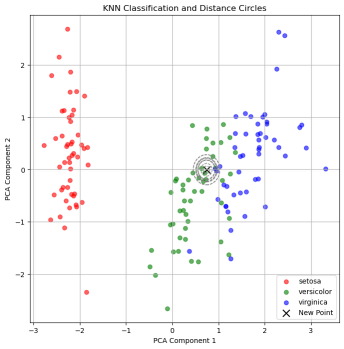
[选读]可视化 KNN

在本案例中，我们使用 KNN 算法来解决鸢尾花分类问题。KNN 算法是一个简单而有效的分类算法，它通过计算样本之间的距离来确定新样本的类别。KNN 算法的优点是简单、易于理解、易于实现、无参数调整，缺点是容易受到样本扰动的影响。

我们可以对某一次预测的过程进行可视化，来更直观地理解 KNN 算法的工作原理：

python

import numpy as np
import matplotlib.pyplot as plt
from sklearn.datasets import load_iris
from sklearn.neighbors import KNeighborsClassifier
from sklearn.preprocessing import StandardScaler
from sklearn.decomposition import PCA

# 加载Iris数据集并标准化
iris = load_iris()
X = iris.data
y = iris.target

scaler = StandardScaler()
X_scaled = scaler.fit_transform(X)

# 使用PCA将数据降维到2D，便于可视化
pca = PCA(n_components=2)
X_pca = pca.fit_transform(X_scaled)

# 训练KNN模型
knn = KNeighborsClassifier(n_neighbors=10)
knn.fit(X_pca, y)

# 选择一个新点进行预测
new_point = np.array([[4.9, 3.2, 5.6, 2.3]])
new_point_scaled = scaler.transform(new_point)
new_point_pca = pca.transform(new_point_scaled)
predicted_class = knn.predict(new_point_pca)

# 可视化训练数据
plt.figure(figsize=(8, 8))
colors = ['red', 'green', 'blue']

for i in range(3):
    plt.scatter(X_pca[y == i, 0], X_pca[y == i, 1],
                color=colors[i], label=iris.target_names[i], alpha=0.6)

# 可视化新点
plt.scatter(new_point_pca[0, 0], new_point_pca[0, 1],
            color='black', label='New Point', marker='x', s=100)

# 画出距离圆
distances, indices = knn.kneighbors(new_point_pca)
for i in range(len(indices[0])):
    neighbor_index = indices[0][i]
    distance = distances[0][i]
    neighbor_point = X_pca[neighbor_index]

    circle = plt.Circle((new_point_pca[0, 0], new_point_pca[0, 1]),
                        distance, color='gray', fill=False, linestyle='--')
    plt.gca().add_patch(circle)

# 图例和标题
plt.legend()
plt.xlabel('PCA Component 1')
plt.ylabel('PCA Component 2')
plt.title('KNN Classification and Distance Circles')
plt.grid(True)
plt.show()

输出结果：

[选读]自己动手 - 实现一个简单的线性回归模型

TIP

线性回归基础知识：线性回归简介

案例：波士顿放假预测

python

from sklearn.linear_model import LinearRegression
from sklearn.datasets import fetch_california_housing
from sklearn.model_selection import train_test_split
from sklearn.preprocessing import StandardScaler
from sklearn.metrics import mean_squared_error

# 1.获取数据
data = fetch_california_housing()

# 2.数据集划分
x_train, x_test, y_train, y_test = train_test_split(data.data, data.target, random_state=22)

# 3.特征工程-标准化
transfer = StandardScaler()
x_train = transfer.fit_transform(x_train)
x_test = transfer.transform(x_test)

# 4.机器学习-线性回归(正规方程)
estimator = LinearRegression()
estimator.fit(x_train, y_train)

# 5.模型评估
# 5.1 获取系数等值
y_predict = estimator.predict(x_test)
print("预测值为:\n", y_predict)
print("模型中的系数为:\n", estimator.coef_)
print("模型中的偏置为:\n", estimator.intercept_)
# 5.2 评价(均方误差)
error = mean_squared_error(y_test, y_predict)
print("误差为:\n", error)

某一次的输出：

shell

预测值为:
 [1.41601135 2.00797685 1.02613188 ... 2.1971023  1.91659415 3.03593177]
模型中的系数为:
 [ 0.82591102  0.11445311 -0.26118374  0.30345645 -0.00706501 -0.04153221
 -0.9107612  -0.88255758]
模型中的偏置为:
 2.069981627260431
误差为:
 0.4918267761529808

完整课程 ​

简介 ​

什么是 sklearn？ ​

sklearn 的主要功能 ​

为什么选择 sklearn？ ​

环境搭建 ​

安装 Anaconda ​

配置环境变量 ​

验证 ​

更改 conda 源 ​

安装相关 Python 库 ​

Hello, Sklearn! ​

机器学习方法 ​

KNN 算法简介 ​

问题分析 ​

数据预处理 ​

划分数据集 ​

训练与预测 ​

模型评估 ​

完整代码 ​

[选读]可视化 KNN ​

[选读]自己动手 - 实现一个简单的线性回归模型 ​

完整课程

简介

什么是 sklearn？

sklearn 的主要功能

为什么选择 sklearn？

环境搭建

安装 Anaconda

配置环境变量

验证

更改 conda 源

安装相关 Python 库

Hello, Sklearn!

机器学习方法

KNN 算法简介

问题分析

数据预处理

划分数据集

训练与预测

模型评估

完整代码

[选读]可视化 KNN

[选读]自己动手 - 实现一个简单的线性回归模型