NumPy 入门

NumPy

什么是 numpy？

Numpy（Numerical Python）是一个开源的 Python 科学计算库，用于快速处理任意维度的数组。

Numpy支持常见的数组和矩阵操作。对于同样的数值计算任务，使用 Numpy 比直接使用 Python 要简洁的多。

Numpy使用 ndarray 对象来处理多维数组，该对象是一个快速而灵活的大数据容器。

ndarray

NumPy 提供了一个 N 维数组类型 ndarray，它描述了相同类型的“items”的集合。

假如我们有如下表格：

numpy-ndarray-table

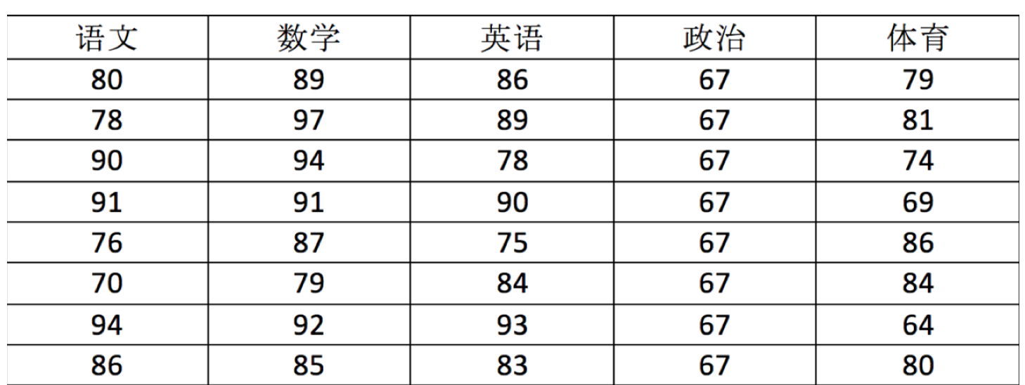
我们可以用 ndarray 进行存储：

python

import numpy as np

# 创建ndarray
score = np.array(
[[80, 89, 86, 67, 79],
[78, 97, 89, 67, 81],
[90, 94, 78, 67, 74],
[91, 91, 90, 67, 69],
[76, 87, 75, 67, 86],
[70, 79, 84, 67, 84],
[94, 92, 93, 67, 64],
[86, 85, 83, 67, 80]])

print(score)

输出结果：

shell

[[80 89 86 67 79]
 [78 97 89 67 81]
 [90 94 78 67 74]
 [91 91 90 67 69]
 [76 87 75 67 86]
 [70 79 84 67 84]
 [94 92 93 67 64]
 [86 85 83 67 80]]

这就是使用 numpy 定义矩阵的基础语法。

[选读]为什么要使用 numpy？

我们使用 Python 的列表就可以存储一维数组，通过列表的嵌套可以实现多维数组，那么为什么还需要使用 Numpy 的 ndarray 呢？

在这里我们通过一段代码运行来体会到 ndarray 的好处:

python

import random
import time
import numpy as np
a = []
for i in range(100000000):
    a.append(random.random())

# 通过%time魔法方法, 查看当前行的代码运行一次所花费的时间
%time sum1=sum(a)

b=np.array(a)

%time sum2=np.sum(b)

其中第一个时间显示的是使用原生 Python 计算时间,第二个内容是使用 numpy 计算时间:

shell

CPU times: user 852 ms, sys: 262 ms, total: 1.11 s
Wall time: 1.13 s
CPU times: user 133 ms, sys: 653 µs, total: 133 ms
Wall time: 134 ms

从中我们看到 ndarray 的计算速度要快很多，节约了时间。

机器学习的最大特点就是大量的数据运算，那么如果没有一个快速的解决方案，那可能现在 python 也在机器学习领域达不到好的效果。

所以，为什么 ndarray 可以做到如此高效的计算呢？

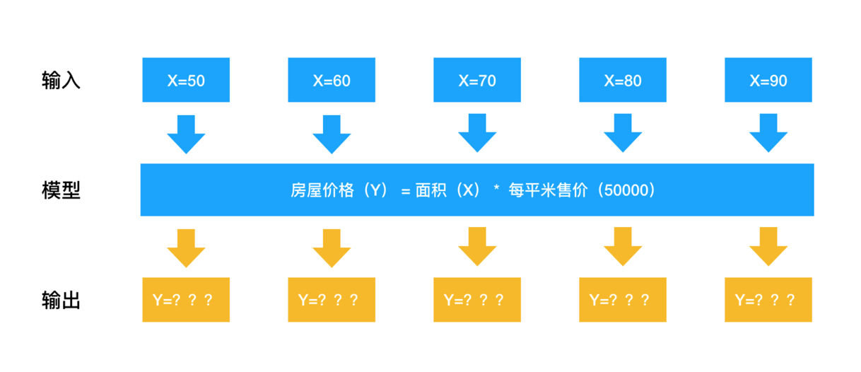
在直观上，numpy 可以并行的计算大量数据，他在某一刻的工作状态看起来可能是这样的：

numpy-ndarray-parallel

Numpy 专门针对 ndarray 的操作和运算进行了设计，所以数组的存储效率和输入输出性能远优于 Python 中的嵌套列表，数组越大，Numpy 的优势就越明显。ndarray 到底跟原生 python 列表有什么不同呢？请看一张图：

numpy-ndarray-compare

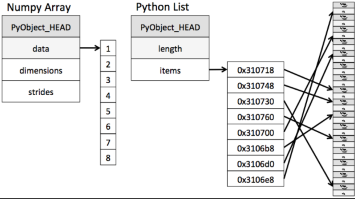
从图中我们可以看出 ndarray 在存储数据的时候，数据与数据的地址都是连续的，这样就给使得批量操作数组元素时速度更快。

这是因为 ndarray 中的所有元素的类型都是相同的，而 Python 列表中的元素类型是任意的，所以 ndarray 在存储元素时内存可以连续，而 python 原生 list 就只能通过寻址方式找到下一个元素，这虽然也导致了在通用性能方面 Numpy 的 ndarray 不及 Python 原生 list，但在科学计算中，Numpy 的 ndarray 就可以省掉很多循环语句，代码使用方面比 Python 原生 list 简单的多。

此外，numpy 内置了并行运算功能，当系统有多个核心时，做某种计算时，numpy 会自动做并行计算。

实际上，之所以 numpy 可以突破 Python 的模式，是因为 Numpy 底层使用 C 语言编写，内部解除了 GIL（全局解释器锁），其对数组的操作速度不受 Python 解释器的限制，所以，其效率远高于纯 Python 代码。（所以 C 永远的神）

N 维数组-ndarray

ndarray 的属性

数组属性反映了数组本身固有的信息。

属性名字	属性解释
ndarray.shape	数组维度的元组
ndarray.ndim	数组维数
ndarray.size	数组中的元素数量
ndarray.itemsize	一个数组元素的长度（字节）
ndarray.dtype	数组元素的类型

ndarray 的形状

首先创建一些数组进行打印：

python

import numpy as np

# 创建数组
a = np.array([[1,2,3],[4,5,6]])
b = np.array([1,2,3,4])
c = np.array([[[1,2,3],[4,5,6]],[[1,2,3],[4,5,6]]])

print(a.shape)
print(b.shape)
print(c.shape)

输出结果：

shell

(2, 3)
(4,)
(2, 2, 3)

可以看到，数组的维度分别为 (2,3), (4,), (2,2,3)，相当于是二维数组、一维数组与三维数组。

如何理解数组的形状？

二维数组：

numpy-ndarray-2d

三维数组：

numpy-ndarray-3d

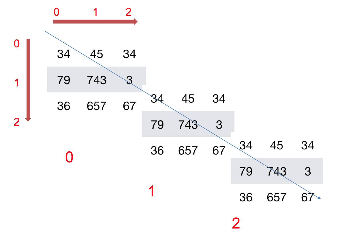
实际上就是一个立方体，维度更多就只能凭想象了

ndarray 的类型

python

print(type(score.dtype))

输出结果：

shell

<type 'numpy.dtype'>

dtype 是 numpy.dtype 类型，先看看对于数组来说都有哪些类型：

名称	描述	简写
np.bool	用一个字节存储的布尔类型（True 或 False）	'b'
np.int8	一个字节大小，-128 至 127	'i1'
np.int16	整数，-32768 至 32767	'i2'
np.int32	整数，-2^31 至 2^32 -1	'i4'
np.int64	整数，-2^63 至 2^63 - 1	'i8'
np.uint8	无符号整数，0 至 255	'u1'
np.uint16	无符号整数，0 至 65535	'u2'
np.uint32	无符号整数，0 至 2^32 - 1	'u4'
np.uint64	无符号整数，0 至 2^64 - 1	'u8'
np.float16	半精度浮点数：16 位，正负号 1 位，指数 5 位，精度 10 位	'f2'
np.float32	单精度浮点数：32 位，正负号 1 位，指数 8 位，精度 23 位	'f4'
np.float64	双精度浮点数：64 位，正负号 1 位，指数 11 位，精度 52 位	'f8'
np.complex64	复数，分别用两个 32 位浮点数表示实部和虚部	'c8'
np.complex128	复数，分别用两个 64 位浮点数表示实部和虚部	'c16'
np.object_	python 对象	'O'
np.string_	字符串	'S'
np.unicode_	unicode 类型	'U'

IMPORTANT

注意：不同版本的 numpy 类型的表示可能不同，比如字符串类型在不同版本的 numpy 中可能是 'S12' 或者 'U12'。

我们在创建数组时可以指定 dtype，也可以不指定，默认是 np.float64：

python

import numpy as np

a = np.array([[1, 2, 3], [4, 5, 6]], dtype=np.float32)
print(a.dtype)

arr = np.array(['python', 'tensorflow', 'scikit-learn', 'numpy'], dtype='|S12')
print(arr)

输出结果：

shell

float32
[b'python' b'tensorflow' b'scikit-learn' b'numpy']

基本操作

创建数组

numpy 提供了多种创建数组的方法。

0 或 1 数组

通过.ones(shape, dtype)、.zeros(shape, dtype)可以创建统一化的 0 或 1 数组：

python

import numpy as np

uni = np.ones([4, 8])
print(uni)

uni = np.zeros([4, 8])
print(uni)

输出结果：

shell

[[1. 1. 1. 1. 1. 1. 1. 1.]
 [1. 1. 1. 1. 1. 1. 1. 1.]
 [1. 1. 1. 1. 1. 1. 1. 1.]
 [1. 1. 1. 1. 1. 1. 1. 1.]]

[[0. 0. 0. 0. 0. 0. 0. 0.]
 [0. 0. 0. 0. 0. 0. 0. 0.]
 [0. 0. 0. 0. 0. 0. 0. 0.]
 [0. 0. 0. 0. 0. 0. 0. 0.]]

根据已有数据生成数组

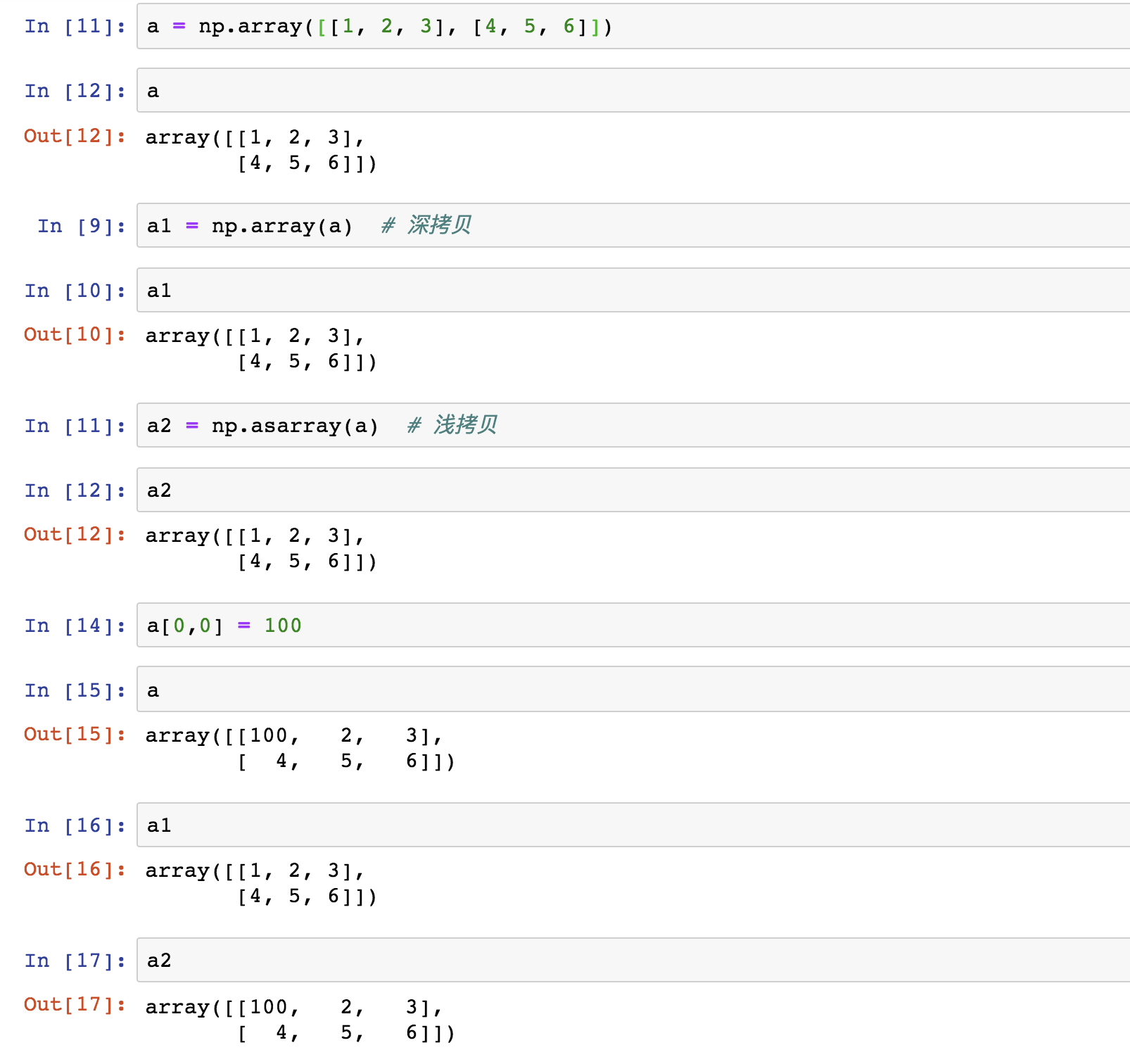
也可以通过现有数组生成，我们之前已经使用过类似的方法：

import numpy as np

a = np.array([[1, 2, 3], [4, 5, 6]])

a1 = np.array(a)  # 从现有的数组当中创建
print(a1)

a2 = np.asarray(a)  # 相当于索引的形式，并没有真正的创建一个新的
print(a2)

输出结果：

shell

[[1 2 3]
 [4 5 6]]

[[1 2 3]
 [4 5 6]]

其区别如下：

numpy-ndarray-create

均分等差数组

python

np.linspace (start, stop, num, endpoint)

其中：

start:序列的起始值
stop:序列的终止值
num:要生成的等间隔样例数量，默认为 50
endpoint:序列中是否包含 stop 值，默认为 ture

例如：

python

import numpy as np

a = np.linspace(0, 100, 11)
print(a)

输出结果：

shell

[  0.  10.  20.  30.  40.  50.  60.  70.  80.  90. 100.]

定长等差数组

python

np.arange(start, stop, step, dtype)

其中：

start:序列的起始值
stop:序列的终止值，不包括在序列中
step:序列的步长
dtype:数组元素的类型，默认为 None

例如：

python

import numpy as np

a = np.arange(1, 10, 2)
print(a)

输出结果：

shell

[1 3 5 7 9]

等比数组

python

np.logspace(start, stop, num, endpoint, base)

其中：

start:序列的起始值
stop:序列的终止值
num:要生成的等间隔样例数量，默认为 50
endpoint:序列中是否包含 stop 值，默认为 ture
base:序列的底数，默认为 10

例如：

python

import numpy as np

a = np.logspace(0, 2, 3)
print(a)

输出结果：

shell

[  1.  10. 100.]

随机生成数组

numpy 提供了许多“随机”的模式，最常用的是正态分布随机与均匀分布随机。

python

np.random.normal(loc, scale, size)
np.random.uniform(low, high, size)

其中：

loc: 均值，默认为 0
scale: 标准差，默认为 1
size: 输出数组的形状，默认为 None

例如：

python

import numpy as np

# 正态分布随机
a = np.random.normal(0, 1, [3, 4])
print(a)

# 均匀分布随机
b = np.random.uniform(0, 1, [3, 4])
print(b)

某次的输出结果：

shell

[[-0.93221265 -0.67635989  0.46675785  0.9485074 ]
 [ 0.41596084 -0.5660286  -0.45686209 -0.70542995]
 [ 0.98862117  0.23921517 -1.14934301  0.94451928]]

[[0.2734833  0.30231068 0.27333733 0.5394391 ]
 [0.9147523  0.62975983 0.0350036  0.47296369]
 [0.14975517 0.00505338 0.64530276 0.09225579]]

数组的索引与切片

在引用数组时，我们可以单独引用某个元素，也可以通过切片的方式引用一部分元素，切片的语法如下：

start:stop:step
start:stop
start:
:stop
:

例如：

python

import numpy as np

a = np.array([[1, 2, 3], [4, 5, 6], [7, 8, 9]])
print(a)

# 单独引用某个元素，索引从 0 开始
print(a[1, 2])  # 6

# 切片，索引从 0 开始，至 end 之前一位结束
print(a[1:3, 1:3])  # [[5 6] [8 9]]

输出结果：

shell

[[1 2 3]
 [4 5 6]
 [7 8 9]]

6

[[5 6]
 [8 9]]

形状修改

形状修改可以改变数组的形状，但不能改变元素的数量。

reshape

返回一个具有相同数据域，但 shape 不一样的视图
行、列不进行互换

python

ndarray.reshape(shape, order)

其中：

shape: 目标形状
order: 排列顺序，默认为 C（行优先）

例如：

python

import numpy as np

a = np.array([[1, 2, 3], [4, 5, 6], [7, 8, 9]])
print(a.shape)  # (3, 3)
print(a)

b = a.reshape([9, 1])
print(b.shape)  # (9, 1)
print(b)

输出结果：

shell

(3, 3)
[[1 2 3]
 [4 5 6]
 [7 8 9]]

(9, 1)

[[1]
 [2]
 [3]
 [4]
 [5]
 [6]
 [7]
 [8]
 [9]]

resize

修改数组本身的形状（需要保持元素个数前后相同）
行、列不进行互换

python

ndarray.resize(shape, refcheck)

其中：

shape: 目标形状
refcheck: 是否检查数组是否为视图，默认为 True

例如：

python

import numpy as np

a = np.array([[1, 2, 3], [4, 5, 6], [7, 8, 9]])
print(a.shape)  # (3, 3)
print(a)

a.resize([9, 1])
print(a.shape)  # (9, 1)
print(a)

输出结果：

shell

(3, 3)
[[1 2 3]
 [4 5 6]
 [7 8 9]]

(9, 1)

[[1]
 [2]
 [3]
 [4]
 [5]
 [6]
 [7]
 [8]
 [9]]

T 转置

数组的转置
将数组的行、列进行互换

python

ndarray.T

例如：

python

import numpy as np

a = np.array([[1, 2, 3], [4, 5, 6], [7, 8, 9]])
print(a.shape)  # (3, 3)
print(a)

b = a.T
print(b.shape)  # (3, 3)
print(b)

输出结果：

shell

(3, 3)
[[1 2 3]
 [4 5 6]
 [7 8 9]]

(3, 3)

[[1 4 7]
 [2 5 8]
 [3 6 9]]

类型修改

astype

返回修改了类型之后的数组

python

ndarray.astype(dtype, order, casting, subok, copy)

其中：

dtype: 目标类型
order: 排列顺序，默认为 K（保持原有顺序）
casting: 类型转换的规则，默认为 unsafe
subok: 是否允许子类，默认为 True
copy: 是否复制，默认为 True

例如：

python

import numpy as np

a = np.array([[1, 2, 3], [4, 5, 6], [7, 8, 9]])
print(a.dtype)  # int64

b = a.astype(np.float32)
print(b.dtype)  # float32

输出结果：

shell

int64
float32

tostring

构造包含数组中原始数据字节的 Python 字节

python

ndarray.tostring(order, sep, dtype)

其中：

order: 排列顺序，默认为 C（行优先）
sep: 分隔符，默认为 None
dtype: 目标类型，默认为 None

例如：

python

import numpy as np

a = np.array([[1, 2, 3], [4, 5, 6], [7, 8, 9]])
print(a.tostring())

输出结果：

shell

b'\x01\x00\x00\x00\x02\x00\x00\x00\x03\x00\x00\x00\x04\x00\x00\x00\x05\x00\x00\x00\x06\x00\x00\x00\x07\x00\x00\x00\x08\x00\x00\x00\t\x00\x00\x00'

数组的去重

python

np.unique(ar, return_index, return_inverse, return_counts)

其中：

ar: 输入数组
return_index: 是否返回下标，默认为 False
return_inverse: 是否返回逆序索引，默认为 False
return_counts: 是否返回计数，默认为 False

例如：

python

import numpy as np

a = np.array([1, 2, 3, 2, 4, 1, 5])
print(a)

b = np.unique(a)
print(b)

c, d = np.unique(a, return_index=True)
print(c)
print(d)

e, f = np.unique(a, return_inverse=True)
print(e)
print(f)

g, h = np.unique(a, return_counts=True)
print(g)
print(h)

输出结果：

shell

[1 2 3 2 4 1 5]
[1 2 3 4 5]
[1 2 3 2 4 1 5]
[0 1 2 3 4 5 6]
[0 1 2 0 3 4 5]
[1 2 3 4 5]
[1 1 1 1 1 1 1]

ndarray 运算

如果想要操作符合某一条件的数据，应该怎么做？

逻辑运算

我们可以通过如下的方法进行逻辑运算：

python

import numpy as np

# 生成10名同学，5门功课的数据
score = np.random.randint(40, 100, (10, 5))
print(score)

# 取出最后4名同学的成绩，用于逻辑判断
test_score = score[6:, ]
print(test_score)

# 逻辑判断, 如果成绩大于60就标记为True 否则为False
test_bool = test_score > 60
print(test_bool)

# 将不及格的同学分数替换为0
test_score[test_score < 60] = 0
print(test_score)

某一次的输出结果：

shell

[[64 72 52 94 45]
 [60 63 67 66 49]
 [56 46 42 65 50]
 [86 46 50 81 43]
 [77 68 86 91 48]
 [43 71 95 79 77]
 [74 80 65 47 42]
 [42 68 80 65 59]
 [65 75 96 96 86]
 [86 69 40 43 47]]

[[74 80 65 47 42]
 [42 68 80 65 59]
 [65 75 96 96 86]
 [86 69 40 43 47]]

[[ True  True  True False False]
 [False  True  True  True False]
 [ True  True  True  True  True]
 [ True  True False False False]]

[[74 80 65  0  0]
 [ 0 68 80 65  0]
 [65 75 96 96 86]
 [86 69  0  0  0]]

通用判断函数

经常使用的函数有：

np.all(a, axis=None, out=None, keepdims=False)：判断数组 a 中所有元素是否都为 True，如果 axis 为 None，则判断所有元素；如果 axis 为整数，则判断指定轴上的所有元素；如果 axis 为元组，则判断指定轴上的所有元素；如果 out 为 None，则返回布尔值；如果 out 为数组，则将布尔值存入 out 数组；如果 keepdims 为 True，则保持维度。
np.any(a, axis=None, out=None, keepdims=False)：判断数组 a 中是否有元素为 True，如果 axis 为 None，则判断所有元素；如果 axis 为整数，则判断指定轴上的所有元素；如果 axis 为元组，则判断指定轴上的所有元素；如果 out 为 None，则返回布尔值；如果 out 为数组，则将布尔值存入 out 数组；如果 keepdims 为 True，则保持维度。

例如：

python

import numpy as np

# 生成10名同学，5门功课的数据
score = np.random.randint(40, 100, (10, 5))
print(score)

# 判断前两名同学的成绩是否全及格
print(np.all(score[0:2, ] >= 60))

# 判断前两名同学的成绩是否有大于90分的
print(np.any(score[0:2, :] > 80))

某一次的输出结果：

shell

[[49 90 97 47 84]
 [98 59 62 96 81]
 [76 68 61 47 83]
 [88 58 92 74 79]
 [42 50 59 79 45]
 [93 72 87 65 76]
 [55 59 74 76 43]
 [99 86 69 66 92]
 [90 98 87 42 51]
 [43 52 56 82 89]]
False
True

三元运算符

通过使用np.where能够进行更加复杂的运算，复合逻辑需要结合np.logical_and与np.logical_or使用，例如：

python

import numpy as np

# 生成10名同学，5门功课的数据
score = np.random.randint(40, 100, (10, 5))
print(score)

# 判断前四名学生前四门课程中，成绩中大于60的置为1，否则为0
test_score = score[:4, :4]
print(test_score)
print(np.where(test_score > 60, 1, 0))

# 判断前四名学生,前四门课程中，成绩中大于60且小于90的换为1，否则为0
print(np.where(np.logical_and(test_score > 60, test_score < 90), 1, 0))

# 判断前四名学生,前四门课程中，成绩中大于90或小于60的换为1，否则为0
print(np.where(np.logical_or(test_score > 90, test_score < 60), 1, 0))

某一次的输出结果：

shell

[[95 89 55 63 73]
 [57 60 79 81 51]
 [67 56 47 67 50]
 [86 45 61 44 71]
 [63 44 75 66 65]
 [96 79 66 90 95]
 [50 40 75 44 40]
 [80 67 42 92 59]
 [43 45 46 48 91]
 [96 56 84 45 81]]

[[95 89 55 63]
 [57 60 79 81]
 [67 56 47 67]
 [86 45 61 44]]

[[1 1 0 1]
 [0 0 1 1]
 [1 0 0 1]
 [1 0 1 0]]

[[0 1 0 1]
 [0 0 1 1]
 [1 0 0 1]
 [1 0 1 0]]

[[1 0 1 0]
 [1 0 0 0]
 [0 1 1 0]
 [0 1 0 1]]

统计运算

如果想要知道学生成绩最大的分数，或者做小分数应该怎么做？

numpy 提供了以下统计函数：

np.max(a, axis=None, out=None, keepdims=False)：返回数组 a 中元素的最大值，如果 axis 为 None，则返回所有元素的最大值；如果 axis 为整数，则返回指定轴上的元素的最大值；如果 axis 为元组，则返回指定轴上的元素的最大值；如果 out 为 None，则返回最大值；如果 out 为数组，则将最大值存入 out 数组；如果 keepdims 为 True，则保持维度。
np.min(a, axis=None, out=None, keepdims=False)：返回数组 a 中元素的最小值，如果 axis 为 None，则返回所有元素的最小值；如果 axis 为整数，则返回指定轴上的元素的最小值；如果 axis 为元组，则返回指定轴上的元素的最小值；如果 out 为 None，则返回最小值；如果 out 为数组，则将最小值存入 out 数组；如果 keepdims 为 True，则保持维度。
np.mean(a, axis=None, dtype=None, out=None, keepdims=False)：返回数组 a 中元素的平均值，如果 axis 为 None，则返回所有元素的平均值；如果 axis 为整数，则返回指定轴上的元素的平均值；如果 axis 为元组，则返回指定轴上的元素的平均值；如果 dtype 为 None，则返回浮点数；如果 dtype 为其他类型，则返回指定类型；如果 out 为 None，则返回平均值；如果 out 为数组，则将平均值存入 out 数组；如果 keepdims 为 True，则保持维度。
np.median(a, axis=None, out=None, overwrite_input=False, keepdims=False)：返回数组 a 中元素的中位数，如果 axis 为 None，则返回所有元素的中位数；如果 axis 为整数，则返回指定轴上的元素的中位数；如果 axis 为元组，则返回指定轴上的元素的中位数；如果 out 为 None，则返回中位数；如果 out 为数组，则将中位数存入 out 数组；如果 overwrite_input 为 True，则修改输入数组；如果 keepdims 为 True，则保持维度。
np.std(a, axis=None, dtype=None, out=None, ddof=0, keepdims=False)：返回数组 a 中元素的标准差，如果 axis 为 None，则返回所有元素的标准差；如果 axis 为整数，则返回指定轴上的元素的标准差；如果 axis 为元组，则返回指定轴上的元素的标准差；如果 dtype 为 None，则返回浮点数；如果 dtype 为其他类型，则返回指定类型；如果 out 为 None，则返回标准差；如果 out 为数组，则将标准差存入 out 数组；如果 ddof 为 0，则计算样本标准差；如果 ddof 为 1，则计算总体标准差；如果 keepdims 为 True，则保持维度。
np.var(a, axis=None, dtype=None, out=None, ddof=0, keepdims=False)：返回数组 a 中元素的方差，如果 axis 为 None，则返回所有元素的方差；如果 axis 为整数，则返回指定轴上的元素的方差；如果 axis 为元组，则返回指定轴上的元素的方差；如果 dtype 为 None，则返回浮点数；如果 dtype 为其他类型，则返回指定类型；如果 out 为 None，则返回方差；如果 out 为数组，则将方差存入 out 数组；如果 ddof 为 0，则计算样本方差；如果 ddof 为 1，则计算总体方差；如果 keepdims 为 True，则保持维度。

例如：

python

import numpy as np

# 生成10名同学，5门功课的数据
score = np.random.randint(40, 100, (10, 5))
print(score)

# 找出学生成绩最高的学生
max_score = np.max(score, axis=0)
print(max_score)

# 找出学生成绩最低的学生
min_score = np.min(score, axis=0)
print(min_score)

# 找出学生成绩平均分
mean_score = np.mean(score, axis=0)
print(mean_score)

# 找出学生成绩中位数
median_score = np.median(score, axis=0)
print(median_score)

# 找出学生成绩标准差
std_score = np.std(score, axis=0)
print(std_score)

# 找出学生成绩方差
var_score = np.var(score, axis=0)
print(var_score)

某一次的输出结果：

shell

[[45 70 44 86 69]
 [60 75 41 96 81]
 [73 71 45 57 54]
 [50 71 40 63 84]
 [46 86 80 89 77]
 [98 93 83 76 81]
 [42 90 83 62 78]
 [78 57 47 96 48]
 [98 92 61 65 82]
 [44 69 76 59 41]]

[98 93 83 96 84]
[42 57 40 57 41]
[63.4 77.4 60.  74.9 69.5]
[55.  73.  54.  70.5 77.5]
[20.89593262 11.48216008 17.68049773 14.80844354 15.08144555]
[436.64 131.84 312.6  219.29 227.45]

数组运算

如果将数组看作一个整体，数组运算类似于把数组看作一个矩阵进行相关处理。

数组与数的运算

python

import numpy as np

arr = np.array([[1, 2, 3, 2, 1, 4], [5, 6, 1, 2, 3, 1]])
print(arr)

arr = arr + 1
print(arr)

arr = arr / 2
print(arr)

输出结果：

shell

[[1 2 3 2 1 4]
 [5 6 1 2 3 1]]

[[2 3 4 3 2 5]
 [6 7 2 3 4 2]]

[[1.  1.5 2.  1.5 1.  2.5]
 [3.  3.5 1.  1.5 2.  1. ]]

需要注意的是，numpy 并不支持类似+=的自运算操作

数组与数组的运算

python

arr1 = np.array([[1, 2, 3, 2, 1, 4], [5, 6, 1, 2, 3, 1]])
arr2 = np.array([[1, 2, 3, 4], [3, 4, 5, 6]])

上面这个能进行运算吗，结果是不行的！

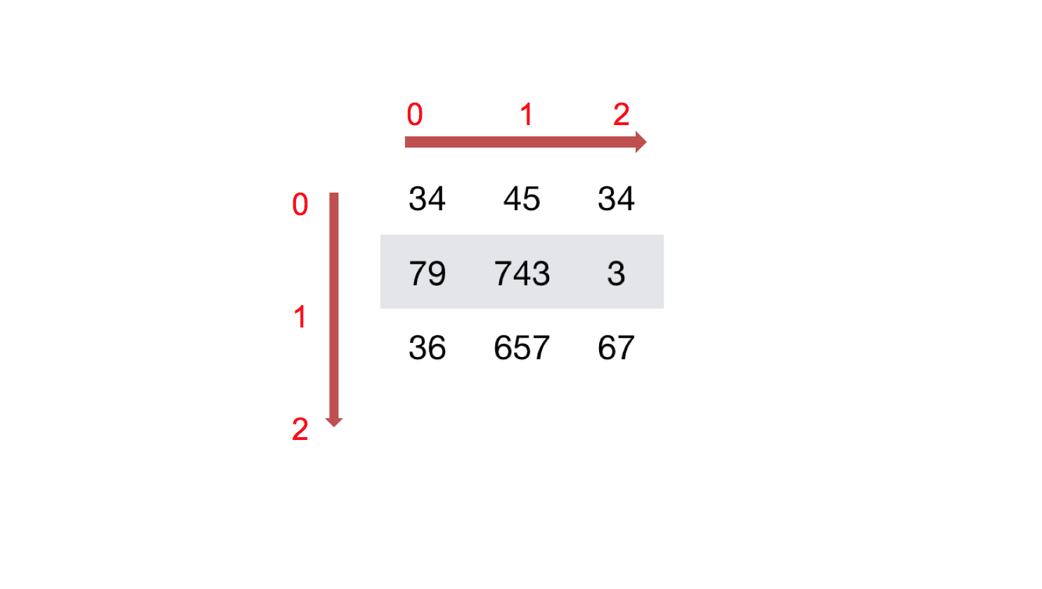
广播机制

数组在进行矢量化运算时，要求数组的形状是相等的。当形状不相等的数组执行算术运算的时候，就会出现广播机制，该机制会对数组进行扩展，使数组的 shape 属性值一样，这样，就可以进行矢量化运算了。

实际上就是线代里面的广播矩阵，如下图所示：

numpy-ndarray-broadcasting

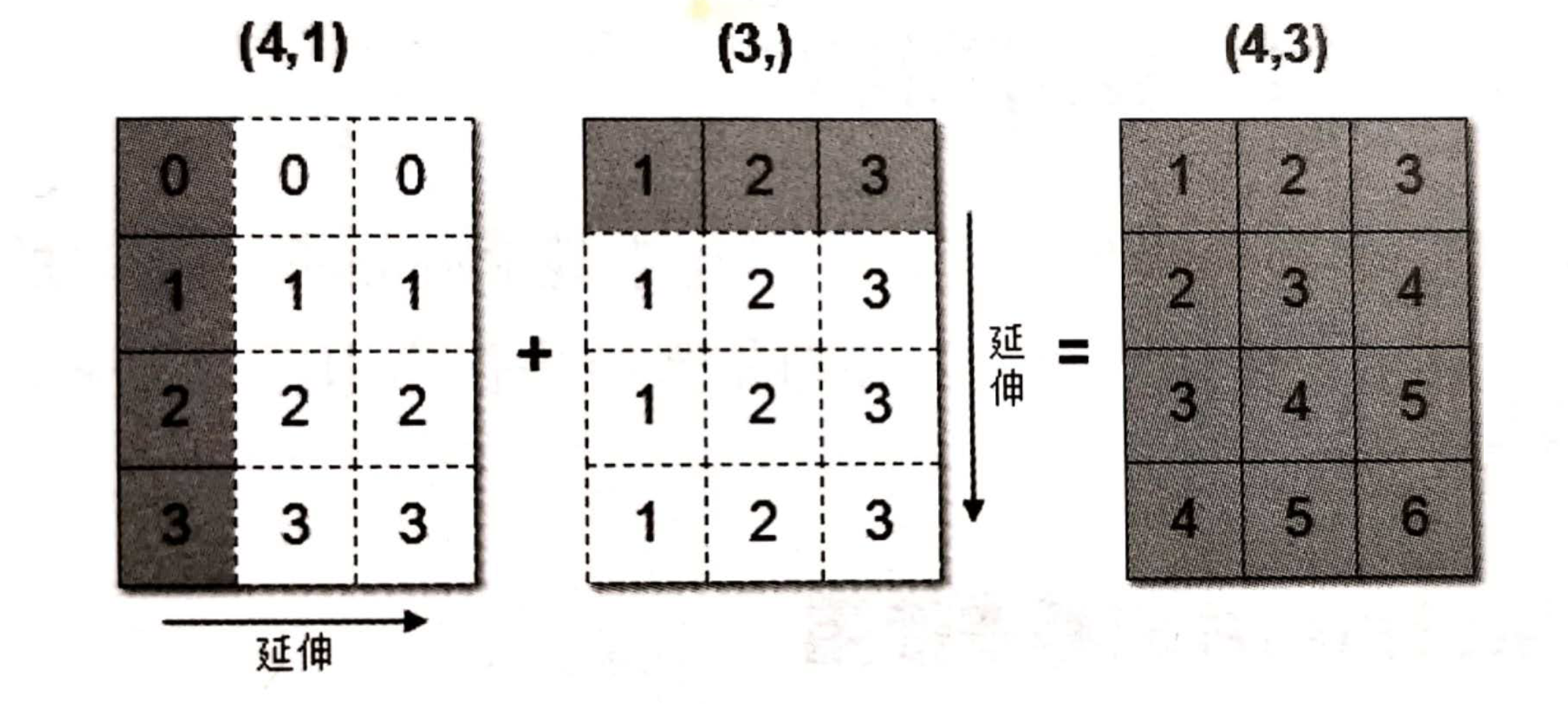
在 numpy 中，广播机制实现了时两个或两个以上数组的运算，即使这些数组的 shape 不是完全相同的，只需要满足如下任意一个条件即可。

数组的某一维度等长。
其中一个数组的某一维度为 1 。

广播机制需要扩展维度小的数组，使得它与维度最大的数组的 shape 值相同，以便使用元素级函数或者运算符进行运算。

需要注意的是，广播机制不意味着矩阵运算，而是数组运算。

例如，这样的数组就可以进行数组间的运算：

python

import numpy as np

arr1 = np.array([[0], [1], [2], [3]])
print(arr1.shape)
print(arr1)

arr2 = np.array([1, 2, 3])
print(arr2.shape)
print(arr2)

arr3 = arr1 + arr2
print(arr3.shape)
print(arr3)

输出结果：

shell

(4, 1)
[[0]
 [1]
 [2]
 [3]]

(3,)
[1 2 3]

(4, 3)
[[1 2 3]
 [2 3 4]
 [3 4 5]
 [4 5 6]]

(4, 3)
[[0 0 0]
 [1 2 3]
 [2 4 6]
 [3 6 9]]

矩阵（向量）运算

矩阵操作需要使用 numpy 提供的运算函数，如dot()、cross()、linalg.inv()等，例如：

python

import numpy as np

# 矩阵点乘
arr1 = np.array([[1, 2, 3], [4, 5, 6]])
arr2 = np.array([[7, 8], [9, 10], [11, 12]])
print(np.dot(arr1, arr2))

# 向量叉乘
arr4 = np.array([1, 2, 3])
arr5 = np.array([4, 5, 6])
print(np.cross(arr4, arr5))

# 矩阵求逆
arr3 = np.array([[1, 2], [3, 4]])
print(np.linalg.inv(arr3))

输出结果：

shell

[[ 58  64]
 [139 154]]

[-3  6 -3]

[[-2.   1. ]
 [ 1.5 -0.5]]

结语

以上就是 numpy 在机器学习中常用的一些方法，希望对你有所帮助！

NumPy 入门 ​

NumPy ​

什么是 numpy？ ​

ndarray ​

[选读]为什么要使用 numpy？ ​

N 维数组-ndarray ​

ndarray 的属性 ​

ndarray 的形状 ​

ndarray 的类型 ​

基本操作 ​

创建数组 ​

0 或 1 数组 ​

根据已有数据生成数组 ​

均分等差数组 ​

定长等差数组 ​

等比数组 ​

随机生成数组 ​

数组的索引与切片 ​

形状修改 ​

reshape ​

resize ​

T 转置 ​

类型修改 ​

astype ​

tostring ​

数组的去重 ​

ndarray 运算 ​

逻辑运算 ​

通用判断函数 ​

三元运算符 ​

统计运算 ​

数组运算 ​

数组与数的运算 ​

数组与数组的运算 ​

广播机制 ​

矩阵（向量）运算 ​

结语 ​

NumPy 入门

NumPy

什么是 numpy？

ndarray

[选读]为什么要使用 numpy？

N 维数组-ndarray

ndarray 的属性

ndarray 的形状

ndarray 的类型

基本操作

创建数组

0 或 1 数组

根据已有数据生成数组

均分等差数组

定长等差数组

等比数组

随机生成数组

数组的索引与切片

形状修改

reshape

resize

T 转置

类型修改

astype

tostring

数组的去重

ndarray 运算

逻辑运算

通用判断函数

三元运算符

统计运算

数组运算

数组与数的运算

数组与数组的运算

广播机制

矩阵（向量）运算

结语